War Story: Porting an Unstable Fortran Program
Programmers tend to tell each other war stories, i.e. stories of a special one of their never-ending fights against complexity. Here is one I can share with the hope that co-programmers in similar situtations might learn something.
The Project
A company asked me to port an old Fortran 90 program to Java. Their last Fortran programmer who was one of the contributors to the program had already retired, and they had no more programmers who were fluent in Fortran. But the program’s results were of high importance, and they wanted to improve it further.
I may not disclose any details of the program, but it was performing some complex physical algorithms and calculations. Basically the program read a few input files which set up parameters, and wrote back a few output files, some with curve data and some just defining one single value.
The program was divided in a dozen Fortran files, all together nearly 10,000 lines long, and my task was not only to just port it, but port it to nice Java. One of my own goals was that the Java port should run with at least half the speed of the original.
I have programmed a bit of Fortran many years ago, and studied Physics, so I was quite a good fit for the task. They provided me with some two dozen input file combinations for testing.
Agenda
My agenda was
- Port the Fortran code directly line by line to Java.
- Check whether that creates the same results, if not fix the bugs. The idea is that if necessary I could debug parallel line by line in both Fortran and Java until I see where I introduced a difference.
- Refactor the result until it is nice Java. Again just check if this produces the same results.
Simple enough, and as always too simple because it didn’t take care of potential problems.
Problems
Basically the Fortran code was awful. It became obvious fast that the engineers that had participated in adding to the code over decades did not know Fortran or programming in general all to well. Most code was copied from long-lost text books (sometimes several times with small differences, probably by different programmers).
The code used hardcoded constants a lot, and often only single-precision (32bit) floating point values. The latter
accidentally, as the default for a floating point constant in Fortran is single precision, and you have to add a suffix
to make it double precision (64bit). This is exactly the opposite of Java where 3.14 is double precision and
3.14f is single precision. Accidentally because all variables were double precision.
E.g. pi was defined over and over as
DOUBLE PRECISION, PARAMETER :: PI = 3.1415926535
This is bad for more than one reason. As said this defines a double precision value from a single-precision constant.
Furthermore, the constant is wrong, the last digit should have been rounded up as the next unshown digit is an 8. But
because that is interpreted as a single precision constant by the compiler the value really used for pi is 3.1415927410125732
which already differs from Math.PI in the 8th digit (at the 6 in the original constant,
also compare π = 3.14159265358979...).
Obviously I wanted to use better precision values for these constants, but in order to be able to compare results
(see agenda 2.) I had to tweak my code that it used either 32bit or 64bit constants. Some physical constants had
improved values nowadays, too. I introduced a global boolean constant COMPATIBLE which was set from
a Java property, and depending on its value I either used the values of the old Fortran program or improved ones.
I also encountered a few bugs during my line-by-line port, so I had to add another constant BUG_COMPATIBLE.
Mainly because I wanted to differ between fixed inaccuracies and fixed bugs.
I found various places where during porting I accidentally used a double precision constant, but my port did still create different results. Because of millions of loops the program was performing it became more and more difficult to find the place where a difference was introduced. Indeed, I had a case were the first difference was happening in the 120,000th loop.
Two things became clear:
- the program was using ill-conditioned
calculations where a small error can make large differences.
E.g. the resulting curves were expected to
be smooth for physical reasons, but sometimes showed chaotic behavior by wildly zig-zagging up and down.
This is usually a sign for chaotic behavior (unavoidably resulting from non-linear equations) or a bad
condition number. - Java did not always get the same results from the same calculation. Sometimes there was a minor difference in the least significant bit.
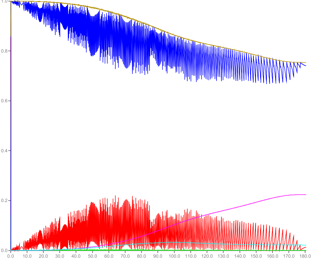
Curves expected to be smooth
Both problems together meant that my calculations would never produce the same results as the original code.
I did a few experiments to fix the second problem like experiencing with strictfp, but that did not help.
It made some calculations perform equal to Fortran, but moved the problem to others.
Sometimes a different algorithm can avoid ill conditions, but that was no option here as it would require to change the basic Fortran program.
And as I had a bunch of refactorings waiting it was clear that I could not keep the current evaluation order of all calculations. But that would also introduce differences:
  double a1 = 3.0 * 2.0 / 5.0;
  double a2 = 3.0 * (2.0 / 5.0);
  double da = a1 - a2;
  assert da == -2.220446049250313E-16;  // true!
Both a1 and a2 should have the same value 1.2 thanks to math, but in reality they will not always be the same
because of the restrictions of floating point handling in computers (like in the example above where da should be 0).
During refactoring I’d expect that there are cases where
I would e.g. refactor the calculation of 2.0/5.0 into another class and use the result. One thing I had
in mind was introducing classes for length and temperature, as the program was mixing meters, centimeters, and
millimeters, as well as °C and K, and in the Fortran program you never knew what was used.
These dedicated classes would definitely change calculations like the above.
Standard test tools which are expecting equal results would not help, and as errors might raise as high as 100% even checks using arbitrary epsilons wouldn’t help, either.
Solutions
Fortran to Java
The solution that I came up with was quite a bit of work. In each Fortran ‘function’ or ‘procedure’ (the Fortran term for a void function, i.e. a function with no return value) of interest I’d dump out the incoming data when the function was entered and the outgoing data when the function was left in each call (or using a fix stepping to avoid flooding my disk). Java would read these dumps, call the equivalent method with the same input data, and look if it reproduces the output data.
My hope was that during one function call the unavoidable differences should not accumulate too much, and I could step through both Java and Fortran in the debugger in parallel, and see where a difference is introduced.
This worked quite well, and depending on the difference which happened I could usually guess whether it
was one of the single/double precision problems (relative error of some 1e-8), a different floating point
calculation (relative error of some 1e-14), or a real bug (larger errors).
Java Refactorings
Having done the line-by-line port from Fortran I had to face the same problem which each refactoring step: did I introduce a bug or is it just some accumulated floating point difference. As this worked well a similar solution seemed the way to go.
But I hated the idea of peppering my code with dumping instruction in every method. It would have been nice if I could avoid the inevitable performance hit, and indeed this is possible. Alas, again it was a lot of work.
Annotations, Class Instrumentation, Bytecode Inspection, and Reflection, and ClassLoaders
The idea was to annotate the methods of interest with a @Dump annotation (allowing a few parameters for tweaking),
and let everything else automatically.
This seems impossible. But Java allows to register a handler for class files which will be called with the binary
data of a class after that is loaded, but before it is converted into the actual Java class object. In this stage
it is possible to instrument the class code (simple example).
In this special case methods with a @Dump instrumentation will get additional bytecode which dumps the input
and output data.
It is important to note that this does not only mean the methods parameters and return value,
but also the this object for a non-static method, and all global variables which the method itself and methods called
by it might use.
The latter made it necessary to decode the bytecode of the method to see which global variables are accessed. At the beginning all methods called (recursively) where also analyzed, but in the end it was more efficient to let this information bubble up. I.e. all methods on the stack were informed about global variables used by the current method.
I used ASM for the class and bytecode handling, although I’m not all too happy with it because at least for me, I had a hard time tweaking it to what I wanted. Luckily I had a bit of experience with Java bytecode from a former project where I implemented my own class reader.
Replaying the dumps was also done automatically. A dump file was read, Java reflection was used to set up the input data and call the method, then expected result and actual result were compared. To make this run faster, this was done multithreaded. Again this was a bit more complex and required dedicated class loaders to allow having a single global object more than once.
Generations
The above worked nicely, and fast SSDs made it even run fast enough to be perfectly usable (60 minutes for a complete dump with all test data, 20 minutes to replay everything). My first dumps and replays with Fortran/Java took days until I sped things up a bit.
But one last problem was left: after a refactoring the information in a dump might no longer match the signature of the new method. It might have gotten another name, more or less or different parameters. So I also introduced dumping generations. A generation was loosely just a set of unchanged method signatures and global variable setting. When that was changed, dumps had to be adapted to be still useful, which was done by a generation adapter. That was a class which got the dumped data and could reorganize it to make it fit for the new setup.
Mostly that could be done in a format where the data was already digested, but sometimes it was necessary to tweak the JSON dump data directly in a first step.
So the final refactoring loop looked like:
- Perform the actual refactoring.
- Write a generation adapter which knows how to fix the dumps from the previous generation to make it fit for the refactored code.
- Run the replay with the adapted dumps from the last generation. Fix all problems and rerun until fixed.
- Write out new dumps with an increased generation.
Conclusion
I have never been that wrong with my estimates before. My customer rented me in 200h blocks, with the idea that after the first there might be one more which would not be completely used. In the end it required 700h of work, and I was happy that my customer was understanding the above problems well, and knew that I was not just playing for time.
Final Java code lines including comments count some 45,000, or without comments some 12,000 (including all dumping code). In the end everything burns down to just 14 ported Fortran lines per hour, or more than 4 minutes porting time per line.
Due to some improved algorithms the Java port usually runs faster than the old Fortran code. Fortran wins for very short runs because the JVM needs a bit of startup time.